
In a previous post we saw how Monte Carlo simulations increase the usefulness of your model in making good decisions in an uncertain world, by incorporating the variability of input assumptions. In this post we’ll look at how to actually build a Monte Carlo simulation. There are plenty of tools out there, but we’ll use a Microsoft Excel add-in called Argo from Booz Allen Hamilton (because it’s free, does the job and leverages Excel, which most business users are familiar with ).
Install Argo
Argo installation is pretty straightforward and takes just 5-10 minutes.
Download Argo for free from https://github.com/boozallen/argo/releases. Make sure to download the 64-bit version if you have a 64-bit system (on a Windows computer you can find out your system type by pressing Windows key+S, typing “about” in the search bar, selecting the “About your PC” option, and seeing what it says under “System type”).
Double-click the downloaded exe file to run it. You’ll be prompted for an extraction location.
Within Excel, go to File > Options > Add-ins. From the “Manage” drop-down select the “Excel Add-ins” option and press “Go”.
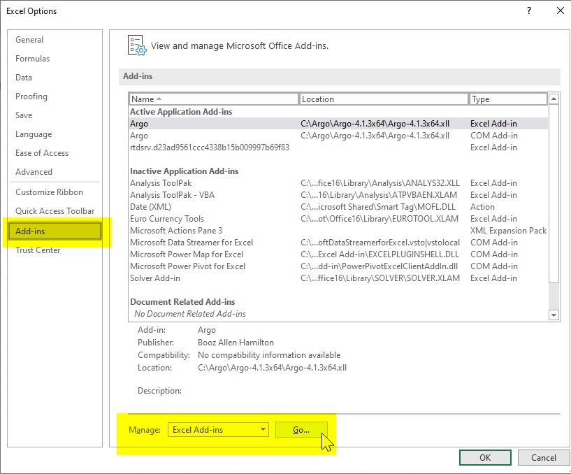
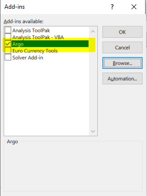
Click on “Browse” and navigate to the extraction location you specified for Argo, and select the .xll file (named something like “Argo-4.1.3×64.xll”, though the exact name may be different if you’ve downloaded a different version). You should now see “Argo” in your list of add-ins and it should be checked:
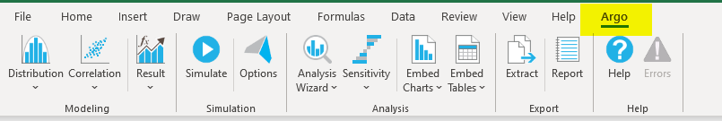
Once you say Ok and go back to Excel you should see a new menu called Argo that looks like this:
Create the plain-vanilla model
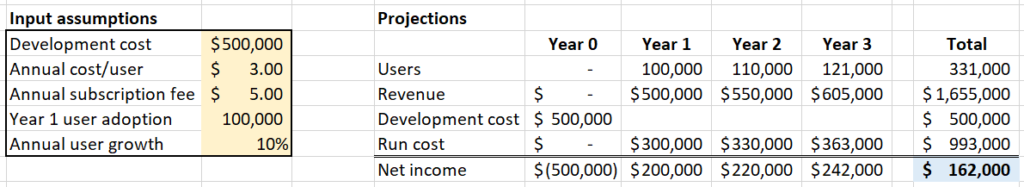
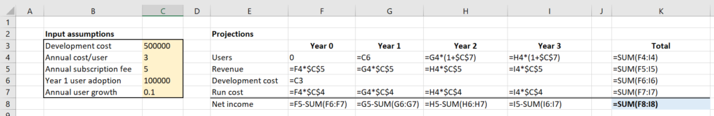
We’ll continue to use the hypothetical example from our previous post, an online subscription service for which we charge a $5 annual subscription fee. We assumed we’d have 100,000 users in our first year and grow our user base 10% each year. It would cost us $500,000 to build, and $3 per user to run. These make up the inputs to our model. Using those inputs we create a four-year projection (with ‘Year 0’ being our investment year):
Here it is with Show formulas toggled on so you can see the relationships between inputs and outputs:
Define probability distributions for your input variables
We’ve got a set of input assumptions that drive our model. In this simplistic model we’ve plugged in single values for each of our inputs (e.g. “$500k development cost”). In the last post we saw that for some inputs we don’t know for sure what the value will be, and we want to be able to factor this uncertainty into our model. We do this by defining a distribution for each uncertain input variable. A distribution is a way to describe the different values that a variable may take, and the likelihood of occurrence of those values.
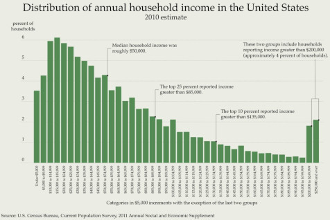
For example, median US household income in 2010 was approximately $50,000. But this distribution of 2010 household income from the US Census Bureau shows us that household income is a range – and if you were to pick a random household in the US, you’re much more likely to pick one with annual income of $20,000 than one with annual income of $150,000.
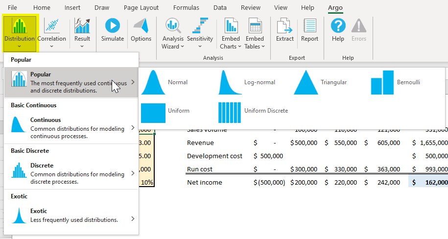
With Argo we can model the uncertainty of our inputs by defining the input variable not as a singe value but as a distribution. We do this by selecting the cell, and in the Argo tab clicking the down chevron of the “Distribution” button and selecting an appropriate distribution.
Here’s where things can get a bit overwhelming: with a multitude of options to choose from, what’s the right/best one to use?
If you’ve been able to collect some data to inform your inputs (maybe performed some surveying, done some sampling, etc), you can plot that data to see what sort of distribution is takes. One of my projects had an input assumption for the time it might take an analyst to perform some task using the product. We mocked up the product screens and had a few analysts perform the task several times under various conditions, and measured time taken, giving us useful data to choose the appropriate distribution parameters.
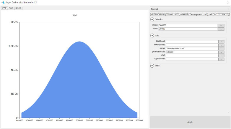
In other situations you may be dependent on a subject matter expert for your inputs. For example, having an engineering manager give you development cost estimates. In such a case you might ask for a “most-likely” estimate along with some upper and lower bound, and use a triangular or trigen distribution. In the image below you can see how Argo shows you the visual distribution of the input variable as you enter in the parameters that describe it. Visualization is a powerful aid, and it’s often helpful to be able to simply sit down with the SME and in real-time tweak the parameters of the distribution to arrive at a spread that they feel comfortable with.
Identify the result cell and run the model
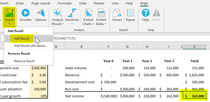
We need to tell the simulation what end result we’re trying to predict. Here we’re interested in total net income over a four-year period (cell K7, highlighted in blue). The cell already has a formula that sums up the net income from years zero through three. With the cell selected, we go to the Argo tab and click on Result > Add result. Notice that doing this wraps the original formula within an @RtaRESULT function.
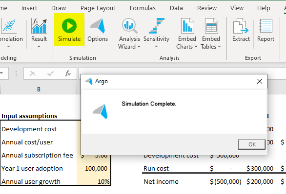
Now press the Simulate button. The time to run the simulation depends on the complexity of the model, specs of your computer and number of iterations being performed, but should generally be just a few seconds or minutes. Once done you’ll get a popup message telling you the simulation is complete.
Let’s take a look at the results!
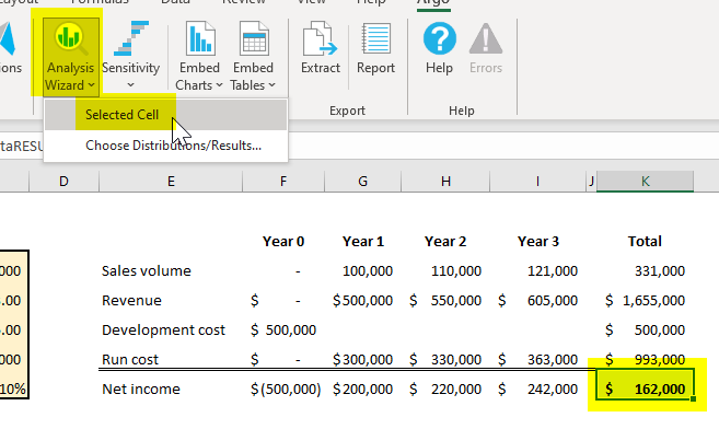
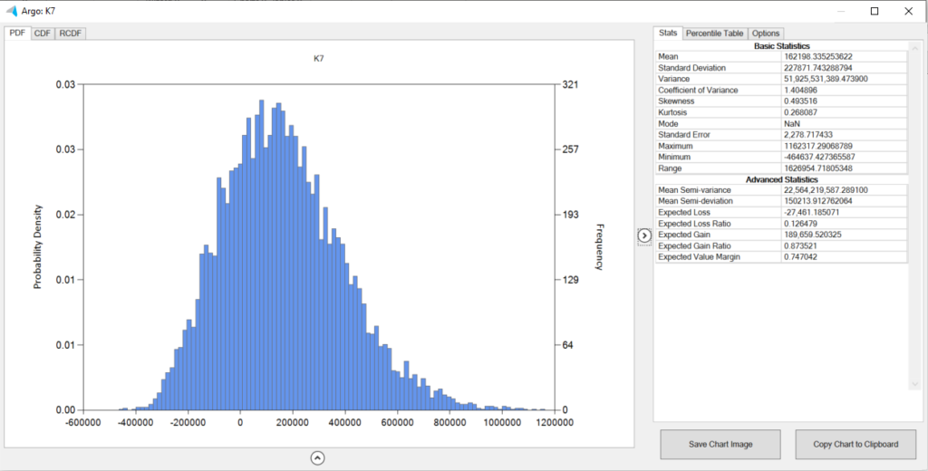
Select the final result cell and click on Analysis Wizard > Selected cell to view a probability distribution of the final result. What this tells you is the range of outcomes you might expect, and the probabilities of those outcomes.
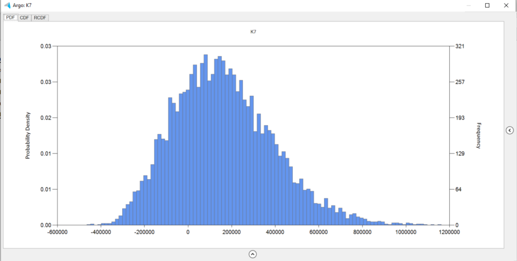
The result that you see here is the outcome of running the model over and over again, computing the result each time for a different set of values for the input variable, those input values being chosen on the basis of the probability distribution we specified for each input. In this way, we are able to compute and visualize a distribution function for the output which is based on the interactions of our variable inputs.
Clicking on the chevron to the right of the distribution opens up a panel showing various statistics related to the distribution.
Closing thoughts
A Monte Carlo simulation allows you to create a more robust predictive model for your product, computing the likelihood of a range of possible outcomes based on variability in inputs.
In my experience, when your inputs are estimates from SMEs they feel more comfortable being able to give you range rather than a single number; Monte Carlo lets you utilize that range.
You can tweak the number of iterations to run the simulation based on the confidence interval and margin of error you are aiming for.
Using this approach will require education within your organization. Though incapable of capturing the nuances of predicting the future, a single number is easier to comprehend; a range of probable outcomes requires more thought. I have had a CFO tell me “This is great, but we can’t put a range into our annual budget so just give me a single number.”
Monte Carlo analysis is not a silver bullet, but it’s certainly a powerful tool to aid in decision-making.